The Water Economics research program hubs collaboration among resource economists and other research disciplines to provide insights on various water uses including agriculture, urban and the environment. Economic costs of drought, policy analysis of water management and their costs are among the span of research produced in the program.
Researchers
Brief Overview of SWAP Model
Statewide Agricultural Production (SWAP) model
This is an introduction to the SWAP Model, the full documentation of the model has been published in The Journal of Environmental Modeling and Software.
The SWAP model is a regional economic model of irrigated agricultural production that simulates the decisions of agricultural producers (farmers) in California. Its data coverage is most detailed in the Central Valley, but it also includes production regions in the Central Coast, South Coast, and desert areas. The model assumes that farmers maximize profit subject to resource, technical, and market constraints. Farmers sell and buy in competitive markets, and no one farmer can affect or control the price of any commodity. The model selects those crops, water supplies, and other inputs that maximize profit subject to constraints on water and land, and subject to economic conditions regarding prices, yields, and costs.
SWAP incorporates project water supplies (SWP and CVP), other local water supplies, and groundwater. As conditions change within a SWAP region (e.g., the quantity of available project water supply increases or the cost of groundwater pumping increases), the model optimizes production by adjusting the crop mix, water sources and quantities used, and other inputs. It also fallows land when that appears to be the most cost-effective response to resource conditions.
When compared to previous PMP based models of irrigated agriculture, SWAP offers three key improvements. First, SWAP includes regional exponential PMP land cost functions, which corrects the inability of previous models, with a quadratic PMP cost function, to handle large policy shocks. Second, SWAP includes regional Constant Elasticity of Substitution (CES) crop production functions which allow for limited substitution between inputs. Leontief production functions were common in many previous models. Finally, regional crop prices are endogenously determined based on a statewide demand function.
Model calibration uses Positive Mathematical Programming (PMP) which has been used in models since the 1980s and was formalized by Howitt (1995). PMP allows the modeler to infer the marginal decisions of farmers while only being able to observe limited average production data through a non-linear cost or revenue function introduced to the model. PMP is fundamentally a three-step procedure for model calibration that assumes farmers optimize input use for maximization of profits. The first step solves a linear profit-maximization program. In addition to basic resource availability and non-negativity constraints, the LP includes a set of calibration constraints to restrict land use to observed values. In the second step, the dual (shadow) values from the calibration and resource constraints are used to derive the parameters for an exponential "PMP" cost function and CES production function. The third step combines the calibrated CES and PMP cost function into a full profit maximization program. The exponential PMP cost function captures the marginal decisions of farmers through the increasing cost of bringing additional land into production (e.g. through decreasing quality). Other input costs, (supplies, land, and labor) enter linearly into the objective function in both the first and third step.
As shown in the image below, the SWAP model has 27 base regions in the Central Valley in addition to agriculture in the Central Coast, South Coast, South Lahontan, and Colorado River regions. There are a total of 37 regions in the current model.

Sequential Calibration and Validation in SWAP
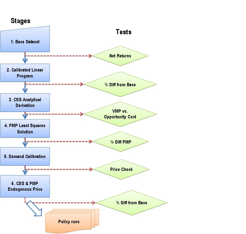
The SWAP model includes a sequential calibration routine and series of validation checks. The calibration phase of the SWAP model uses a sequential six-step process. The six steps are:
- Assemble input, output and elasticity data
- Solve a linear program subject to fixed resource and calibration constraints
- Derive the CES production function parameters using input opportunity costs from step two
- Estimate the crop and region-specific PMP cost functions using a least squares method
- Calibrate the aggregate demand functions and regional adjustment costs using prior demand elasticity estimates, and
- Optimize and simulate the calibrated SWAP model which includes tests for adequate calibration in terms of input and output prices and quantities.


